An article about “FinTech Trends” and an example of the use of R code using Google Trends by Dr. David Krause, AIM Program Director, Marquette University
FinTech has taken the financial
services industry by storm. According to a Google Trends analysis I recently
undertook as of 1/21/2019 - the current interest in FinTech continues to grow
exponentially – not only in the United States, but globally.
As the following chart displays, Interest over time (a Google metric based on search interest – which the reader can think of as an improved version of Google ‘hits’) exploded about five years ago (2014).
Interestingly, as the following chart shows, Interest over time for
both the United States (US) and Japan (JP) also increased about five years ago;
however, the US rate of search interest in FinTech has grown by a greater rate
recently than Japan.
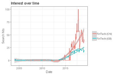
The following chart indicates that both China (CN) and Great Britain (GB)
have had increased FinTech Interest over time; however, both occurred later
than the US and Japan – about 2016 for China. A significant development in
Asian FinTech growth was the high-profile announcement of several major deals:
in 2016 there the deal on Artificial Intelligence (AI) between ChinaAMC, a
Chinese mutual fund and Microsoft - and in 2017 with a major agreement between
the Bank of China and Tencent.
Using Google Trends and R it possible to look
at more recent trends in FinTech Interest over time (the past five years) for the world, US, and China.
The information presented above was obtained from a R code written by David Krause and compiled and viewed using R Studio. The code is contained below:
#Analyzing 'FinTech' in Google Trends with R by David Krause, Marquette AIM Program director
#load the following:
library(gtrendsR)
library(reshape2)
library(ggplot2)
## get web query activity for keyword = "FinTech"
## Different go codes and time can be used.
#Here is a short-cut to run plots of Google Trends search data
plot(gtrendsR::gtrends(keyword = c("FinTech"), time = "all"))
plot(gtrendsR::gtrends(keyword = c("FinTech"), time = "today+5-y"))
#It is possible to look at search times by geography (i.e. United States - US, Japan - JP)
plot(gtrendsR::gtrends(keyword = c("FinTech"), geo = "US", time = "all"))
plot(gtrendsR::gtrends(keyword = c("FinTech"), geo = "US", time = "today+5-y"))
plot(gtrendsR::gtrends(keyword = c("FinTech"), geo = "JP", time = "all"))
plot(gtrendsR::gtrends(keyword = c("FinTech"), geo = "JP", time = "today+5-y"))
res0 = gtrends(c("FinTech"), gprop = "web", time = "all")
plot(res0)+geom_smooth()+geom_line(lwd = 1)
res1 = gtrends(c("FinTech"), gprop = "web", time = "all", geo = c("US"))
plot(res1)+geom_smooth()+geom_line(lwd = 1)
res1a = gtrends(c("FinTech"), gprop = "web", time = "all", geo = c("JP"))
plot(res1a)+geom_smooth()+geom_line(lwd = 1)
res1b = gtrends(c("FinTech"), gprop = "web", time = "all", geo = c("US","JP"))
plot(res1b)+geom_smooth()+geom_line(lwd = 1)
res1c = gtrends(c("FinTech"), gprop = "web", time = "all", geo = c("GB","CN"))
plot(res1c)+geom_smooth()+geom_line(lwd = 1)
res2 = gtrends(c("FinTech"), gprop = "web",time="today+5-y")
plot(res2)+geom_smooth()+geom_line(lwd = 1)
res3 <- c="" font="" geo="c(" gprop="web" gtrends="" intech="" time="today+5-y">
plot(res3)+geom_smooth()+geom_line(lwd = 1)
res3a <- c="" font="" geo="c(" gprop="web" gtrends="" intech="" time="today+5-y">
plot(res3a)+geom_smooth()+geom_line(lwd = 1)
# Get data from Google Trends
#res2a = gtrends(
# c("FinTech"),
#geo = c("US","CN"),
#gprop = "web",
#time = "today+5-y") [[1]]
#define the keywords to analyze from Google Trends
keywords=c("FinTech")
#set the geographic area: (i.e. US = United States, CN = China)
country=c("US","CN")
#set the time window
time=("today+5-y")
#set channels
channel='web'
#access the data from Google Trends
trends = gtrends(keywords, gprop =channel,geo=country, time = time )
#select Google Trends Interest over Time (similar to hits)
time_trend=trends$interest_over_time
#display the first several data items
head(time_trend)
#plot the data items
plot<-ggplot aes="" data="time_trend," x="date," y="hits,group=keyword,col=keyword))+</font">
geom_line()+xlab('Time')+ylab('Relative Interest')+ theme_bw()+
theme(legend.title = element_blank(),legend.position="bottom",legend.text=element_text(size=12))+ggtitle("Google Search Volume")
plot


